Kelp: How to parse logs (without regex)
January 2, 2026
16 min read
by Satyam Singh
The contents of this blog are based on a massive tangent we took while trying to make a metadata pipeline with zeroshot-metadata. Essentially, we were trying to use a small LLM model to answer some yes/no questions to figure out the actual severity of some logs. Despite sinking a lot of time into that, we came to the conclusion that it’s simply not going to be fast enough to keep up with the amount of logs we might generate on average. But what if we put a hashmap on it to cache it? The idea is not bad, but cache on which key? The token processing or something else? Then the idea came up that if we can just get the log template for the message part of the logs, we can make the process several orders faster.
There must be some fantastically fast log parsing algorithm out there that we can use… right? We looked at several of these, but found that each of the algorithms had some good ideas in them which, in practice, were badly flawed.
This might resonate with some of you who have tried some form of log parsing yourself.
We can first start by understanding what even is the main difficulty in log parsing. The first main problem in log parsing is that logs are semi-structured strings of information. Logs are often written with no guidelines attached to them. Logs can come from various sources and have different structures, making it challenging to create a few regexes or a simple parser that can handle most or all cases.
Just to clarify, log parsing is overloaded with two types of “parsing”. One is concerned with converting log lines into a structured struct of sorts, with the complex part tucked away in the message field.
For example, here is an example of logs from a Java server:
2023-10-27 10:00:01.123 INFO [main] com.stonebucklabs.App - Application started successfully.
2023-10-27 10:00:05.456 WARN [http-nio-8080-exec-1] com.stonebucklabs.UserService - User with ID 1234 not found in cache, fetching from DB.
2023-10-27 10:00:10.789 ERROR [task-scheduler-1] com.stonebucklabs.DataProcessor - Failed to process data for batch ID BATCH-001.
2023-10-27 10:00:12.321 DEBUG [http-nio-8080-exec-2] com.stonebucklabs.ProductService - Request received for product sku P-789 region=US category=electronics
Here is the template that most people would want to use for structured storage.
<timestamp> <level> [<thread>] <class> - <message>But we were interested in finding the log template for the message part of the logs so that we could use it to cache the results. For the above example, that should look something like this:
Application started successfully.
User with ID <*> not found in cache, fetching from DB.
Failed to process data for batch ID <*>.
Request received for product sku <*> region=<*> category=<*>
is is a much harder process to automate and is impossible to do manually, because parsers do not know which token inside the message is variable or static. Is 1234 a variable? ( Probably ); Is DB static, or is it a backend name? Are region= and category= part of the template or optional variables?
There are just too many cases, and we realized that existing parsers sometimes rely on regexes to eliminate some of the noise. It’s not a bad strategy, but it’s not perfect either. Another major problem we saw is that if a bad early decision is made by parsers, this can cause bad inference and even something referred to as “template explosion,” as the same type of log events will be grouped on the wrong criteria, causing many template entries instead of a few.
Here are some patterns that generally hold for logs. These are kind of self-evident if you pause and think about them for a bit. We will see these being used in the example ahead.
- Most of the time, there is at least one static token in the message part of the logs.
- The variable parts, being variable, will have more cardinality than static parts.
- There are similar sets of tokens that do vary, but they do not vary enough to be called variables. Additionally, they appear in more than one type of log line. These we call parent tokens (prefixes like
[main],http,ssh, etc.).
Now let’s see how people have approached this problem, with a review and downsides of existing algorithms.
Drain
This parser is the simplest and surprisingly very effective. The first priority of this algorithm is to classify the log messages in clusters based on the length of the message (word count) and by some set of tokens starting from the beginning of the message. The number of tokens it will consider is defined by it's depth parameter. Number of Words in log events is a very effective criteria for splitting the log, because logging statements are almost always just some set of predefined static tokens (a.k.a template) interleaved with dynamic parts. But then how would we know the first token is static or not, here drain takes the first assumption that it will not consider numbers or special characters as viable token for traversal, so they are mapped to a special node to avoid branch explosion ( node with "*" on it in the above diagram ). Variable tokens which are just made of alphabets can still cause the branch explosion problem though but it is considered a tradeoff. The last step is to go to the node and match the supposedly similar logs and replace the difference found with <*>. This is not always reliable as logs that should have two different template can end up in one cluster and the differences in them is just turned into a variable. Despite the downside this is still good enough for most of the use-cases if used correctly.
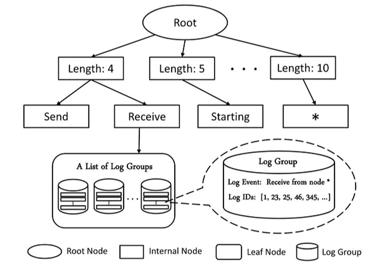
Logram
This is an automated log parsing approach that leverages n-gram dictionaries. Logram stores the frequencies of n-grams in logs and uses them to extract static templates and dynamic variables. It is based on the intuition that frequent n-grams are more likely to represent static templates, while rare n-grams are more likely to be dynamic variables.
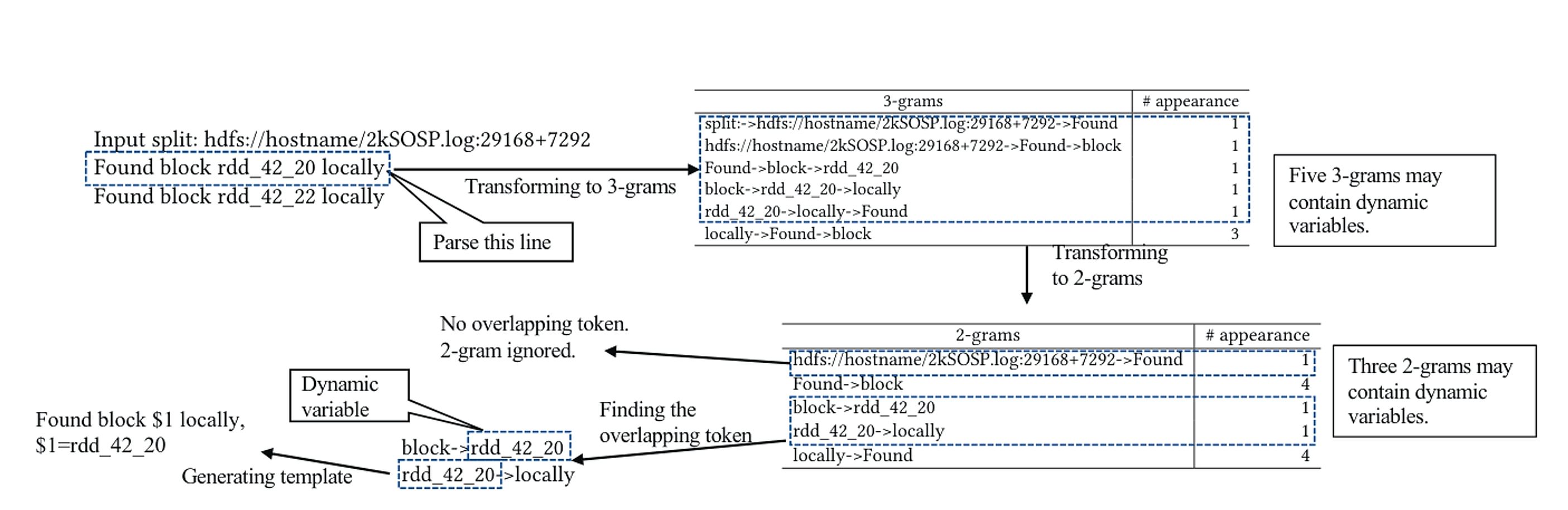
More plainly, if we set n to 3 (the highest n-gram level used), the algorithm generates 3-grams of consecutive words for each log line, wrapping around for the last few tokens, and stores them in a 3-gram dictionary. Based on the dictionary’s state, a threshold is defined below which 3-grams are considered to indicate dynamic positions in the log line. These 3-grams are then broken down into 2-grams and added to a 2-gram dictionary. Again, 2-grams below a threshold are identified, and overlapping parts are compared to infer the dynamic word positions.
This approach works well in many cases but relies on a key assumption: dynamic variables are spaced far enough apart to clearly distinguish static and dynamic parts. Logram fails when dynamic parts sandwich a static part; without additional rules, this can lead to incorrect templates.
Brain
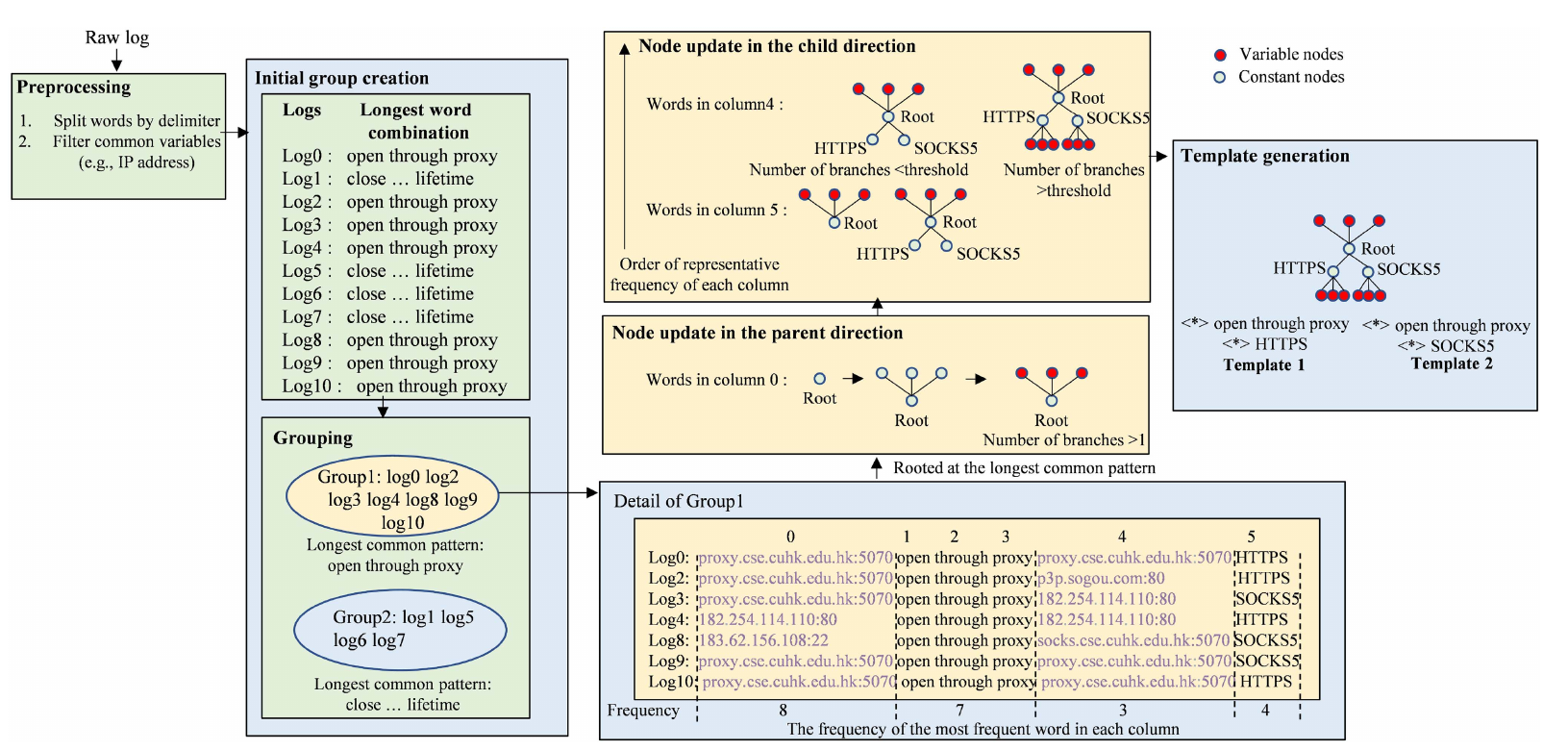
Brain is an offline log parsing algorithm which improves on limitations seen earlier in Drain. Similar to Drain, It starts by grouping logs by length, but then makes a smarter choice for further grouping. Instead of just using the first token to split logs, Brain finds the longest common pattern among all logs in a group. The insight here is that this pattern is very likely to include the static parts of a log template - the parts that stay the same across similar log messages. This longest common pattern then becomes the root of a bidirectional tree. From this root, Brain builds out two directions:
- The parent direction, which adds tokens that appear more frequently (as mentioned before things like
[main],http, etc). - The child direction, rest of the tokens which are less frequent than root. each level in the child direction is placed in increasing order of cardinality.
This hierarchical tree structure allows Brain to gradually grow the template, As the tree branches grow, if any position has too many variations (beyond a set threshold), that position is marked as dynamic <*> in the template.
A major downside of this parser is that it is not streaming, so it requires a large amount of data to be ingested before parsing can begin. Additionally, the bidirectional tree does not preserve the relationship between the root, parent and child nodes, making it difficult to restructure the tree if the initial assumption was incorrect. Finally, rare log patterns often do not occur frequently enough to cross the root selection threshold, leading to missed or incorrect templates.
Kelp
This shows that the parsing problem is not easy and there is no one size fits all solution. Each algorithm has its own tradeoffs and it is important to understand the limitations of each algorithm before using them in production. We don't claim to have solved all the problems but we think kelp can be the go to default parser for most log parsing needs.
We wanted our log parser to be a streaming algorithm like Drain. This is important because we want it to be as easy as a “run and forget” type of deal. Not to mention, it becomes a hassle when someone has to run the algorithm once a day or so to catch any new type of log event flowing through their system. Also, rare log events are harder to extract templates for in an offline parser due to the lack of occurrences in the gathered dataset.
Kelp borrows its steps from Drain and Brain. To start understanding the algorithm, we imagine a set of log lines flowing into the system. Our first job is to segregate them so that the same log event types are placed in the same bucket.
This is where segregating by word/token length is the simplest and most effective choice we can make. But what happens when a dynamic variable position (<*>) is optionally filled or spans multiple tokens? This is the first trade-off: the assumption is that even if log events land in a few different buckets, we will eventually see the same template form across those length buckets.
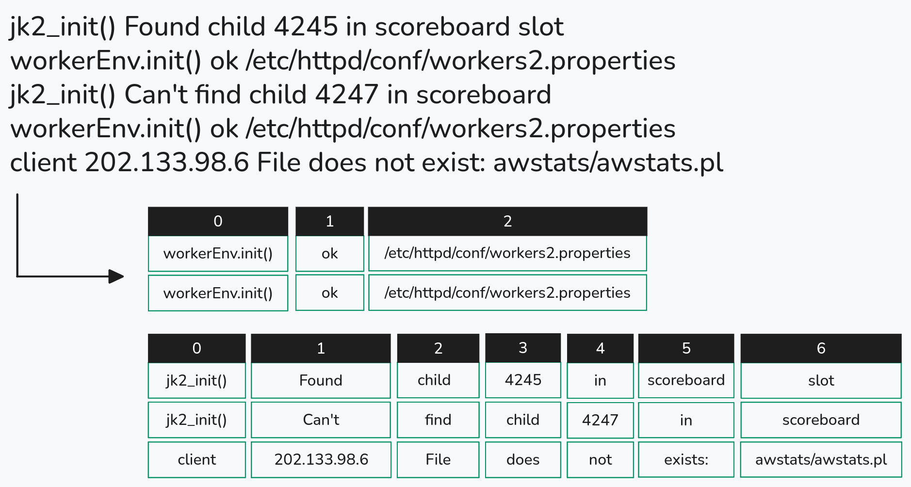
After separating logs by word length, we can represent each log event in a columnar form, meaning we track not just the token but also its position.
So far, so good but how do we further segregate log events within a bucket? Unlike Drain, which assumes the first few tokens are likely static, we wanted something with stronger guarantees. This is where the insight from Brain’s longest common pattern root selection becomes useful. When you look at log lines of the same length side by side, this is what you might notice.
| Request | received | for | product | sku | <*> | region=<*> | category=<*> |
| Failed | to | process | data | to | batch | ID | <*> |
| Request | received | for | product | sku | <*> | region=<*> | category=<*> |
| Request | received | for | product | sku | <*> | region=<*> | category=<*> |
| Failed | to | process | data | to | batch | ID | <*> |
Inside a bucket, a logging statement will always have the same constant words in the same column positions (for example, Request is first and product is always the fourth word). This makes an ideal root choice and removes the need for arbitrary decisions or special cases. But to even find this, we need to keep track of which words appear in which column positions and how often. We can do this using a simple hashmap like structure, which maps (column, token) pairs to their frequency. We refer to this as column–word frequency.
This is where the algorithm differs from Brain. Instead of first building the hashmap with some entries and then segregating logs based on it, we make decisions as the data arrives in order to keep everything streaming.
When a log event arrives in a bucket, we first populate the column–word map. We then update the existing trees in that bucket. Let us assume this is the first log event in the bucket. Since we do not yet know which parts are static and which are dynamic, we place everything at the root for now. We will see shortly how this root evolves into a tree.
When new log lines enter a bucket, the hashmap is updated by incrementing the count for each observed (column, token) pair. A root is intended to represent the longest sequence of static tokens common to a log event type. For example, [Request received for product sku] or [Failed to process data for batch ID] could form valid roots.
To identify a root, we look for (column, token) pairs with the same frequency, since equal frequency suggests those tokens are likely static (ties are broken by choosing the more stable combination). As the map changes, some roots may become invalid if their columns no longer share the same frequency. In such cases, the longest valid sequence is recomputed, and remaining columns are pushed down to child nodes.
Once all roots are validated, new log events are matched against existing roots. If a match is found, the values are added to that tree; otherwise, a new root is created.
After all the complexity of log segregation and root formation, we can now focus on how we ensure a consistent parse tree for template generation. Since Kelp is a streaming algorithm, we can never be fully sure during execution that the current tree is the correct one. To account for this, we retain as much information as possible without wasting memory.
We use three types of nodes: Root, Static, and Dynamic. The Root node was discussed earlier. Static nodes, as the name suggests, represent static tokens that are not part of the root and are used to split the tree when different log event types share a common root. Dynamic nodes represent variable positions (<*>). If a Root or Static does not have a sub-tree, it maintains a count property that tracks how many times that value has been seen.
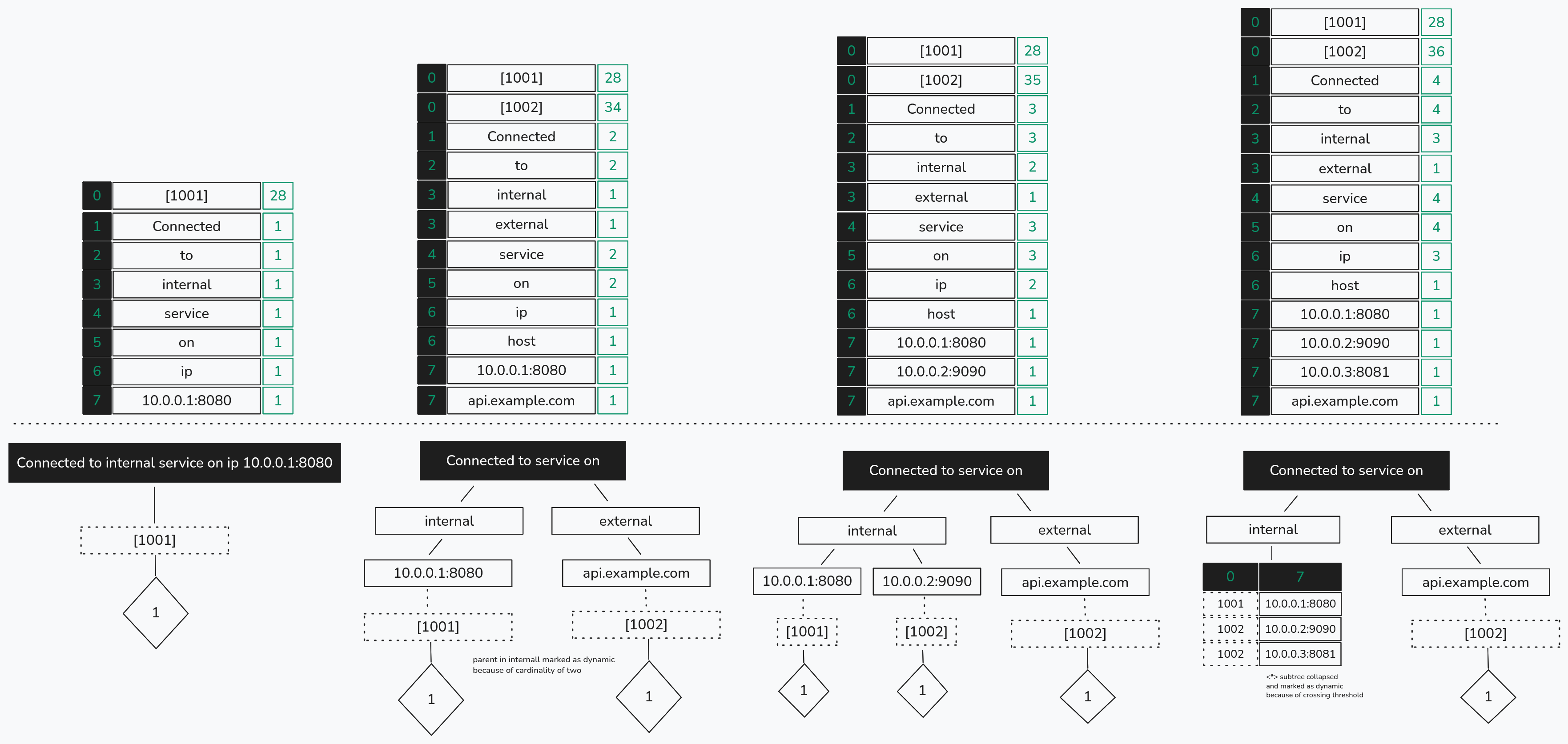
This structure is similar to a trie: duplicate values are merged into static nodes, and traversing the tree from top to bottom yields the set of log events captured by the tree while preserving relationships between (column, token) pairs. A Root can also represent more than one log event type. For example, consider the following made-up log statements.
log("Connected to internal service on ip {}:{}", ip, port);
log("Connected to external service on host {}", hostname);
These two statements are of the same length and share a common root: [Connected to service on]. However, if we simply mark the differences as dynamic (<*>), we would derive an incorrect template:
Connected to <*> service on <*> <*>
This is overly generalized and incorrectly assumes that internal and external are dynamic, when they should instead belong to different clusters with separate templates.
To fix this, when forming a sub-tree at any level below the root, we select the column position with the lowest cardinality. For each distinct token at that position, we create a corresponding node. In the example above, this would result in two child nodes - internal and external - directly under the root, and the original sub-tree is partitioned accordingly.
All of this is done in a streaming manner. If a deeper level of the sub-tree has lower cardinality than the current node, that level is promoted upward and the sub-tree is re-evaluated. This operation is described briefly in our paper.
We have not yet touched on the concept of parent tokens, as mentioned in Brain. To re-illustrate: we may find that some column positions have a higher frequency than the root node itself. We treat these columns as parent positions. Parent positions indicate that a token is not specific to a single log cluster but is common across many different log event types within the same bucket.
log("[ {} ] Connected to internal service on ip {}:{}", thread_id, ip, port);
log("[ {} ] Connected to external service on host {}", thread_id, hostname);
Here, the thread ID is a prefix and appears in all log statements, giving it a higher occurrence count than the message itself. These are what we call parent tokens. Since they are common across log events, they are not useful for forming sub-trees; we want to partition logs by internal and external, not by the value of thread_id - which we already know is dynamic.
However, due to the streaming constraint, we cannot handle parent positions the same way as Brain, where they are placed above the root of a bi-directional tree. We must retain them in case the column–word map later shows a lower frequency for a previously assumed parent column. As a result, parent tokens are not represented by special nodes. Instead, they are placed among child nodes to preserve their relationship with others. Their presence is ignored during sub-tree splitting, and during re-evaluation we ensure they consistently appear at the leaf level.
Benchmarks
In Benchmarks we wanted to put Drain and Logram head to head against Kelp. Here is what we observed. Detailed benchmarks can be found in our paper. We generated Datasets of 15000 lines from set of templates extracted from various datasets in Loghub to create a benchmark where factors such as tokenization strategy and affixes around tokens like () and "" are not a factor. We made this choice because these can be handled separately and does not show the performance of the core of the algorithm
| Parser | Time(s) | Templates Generated | Ground Truth | Grouping Accuracy | Parsing Accuracy |
|---|---|---|---|---|---|
| Drain | 0.40 | 1091 | 180 | 0.790 | 0.766 |
| Logram | 0.65 | 544 | 180 | 0.778 | 0.593 |
| KELP | 0.22 | 207 | 180 | 0.878 | 0.912 |
Across the board we observed a faster runtime and a near accurate Template Generation. Our root is a better strategy for Grouping than what Drain and Logram does, that's why we see much closer numbers to the Ground Truth. We did not put Brain in this as it cannot be used for streaming inference but we would expect a very similar accuracy from Brain if we spent some time picking the right threshold for the dataset.
The code is available here 🌐 in our Codeberg repo you can also expect a official rust and python library and a CLI tool release in near future.
Thanks for sticking through this article, It may be that some concepts overwhelmed and did not make sense or were not clearly explained. If you wish to find out more then please read the paper.